Beyond Classical Search
Local search, continuous optimization, nondeterministic and partial-observation search.
Beyond Classical Search
Chapter [ch:solving-problems-searching] covered search in observable, deterministic, known environments where the solution is a sequence of actions. This chapter relaxes those assumptions. We cover local search algorithms that work on complete-state formulations, methods for nondeterministic and partially observable environments, and online search agents that explore unknown spaces.
Local Search Algorithms and Optimization Problems
Local search algorithms operate on a single current state (or a small number of states) and move only to neighbors. They do not keep paths in memory. This gives two key advantages: very little memory (usually constant) and the ability to find reasonable solutions in large or continuous state spaces where systematic algorithms are unsuitable.
Optimization Problem
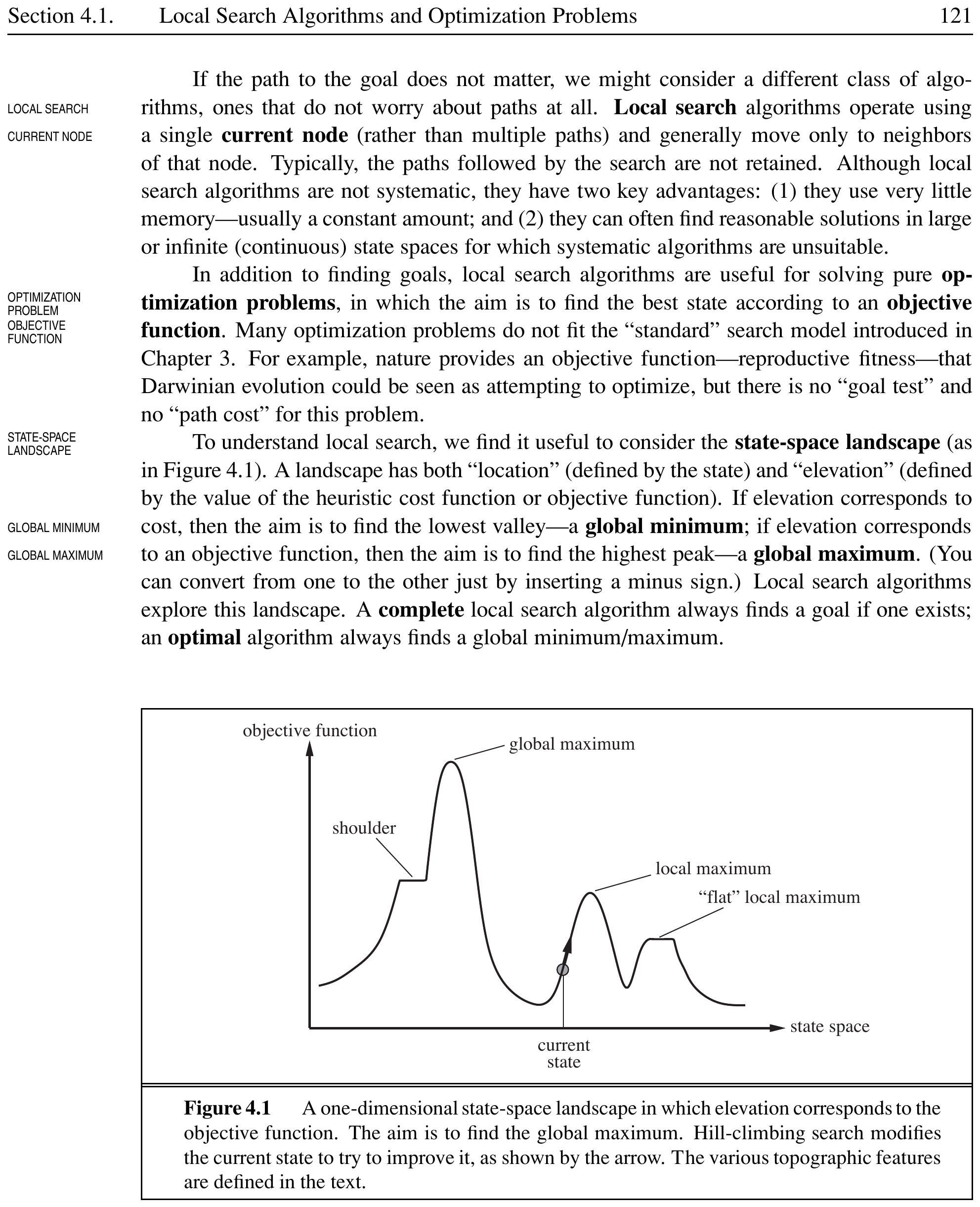
An optimization problem is a problem in which the aim is to find the best state according to an objective function (also called a cost function). The path to the solution does not matter — only the final state. The state-space landscape has locations defined by states and elevation defined by the value of the objective function. A global maximum is the highest peak; a global minimum is the lowest valley.
Hill-Climbing Search
Hill-Climbing Search (Steepest Ascent)
A local search algorithm that continually moves in the direction of increasing value. At each step, it evaluates all neighbors and moves to the best one. It terminates when no neighbor has a higher value than the current state. Also called greedy local search.
Hill-Climbing Pseudocode
1
2
3
4
5
6
7
		function HILL-CLIMBING(problem) returns a state
		current $\gets$ MAKE-NODE(problem.INITIAL-STATE)
		loop do
		neighbor $\gets$ highest-valued successor of current
		if neighbor.VALUE $\le$ current.VALUE then return current.STATE
		current $\gets$ neighbor
Hill climbing does not maintain a search tree. The data structure for the current node needs only the state and the value of the objective function. This resembles trying to find the top of Mount Everest in a thick fog while suffering from amnesia.
Problems that plague hill climbing:
Local maximum: A peak higher than all neighboring states but lower than the global maximum. The algorithm gets stuck here.
Ridge: A sequence of local maxima that is very difficult for greedy algorithms to navigate.
Plateau: A flat area of the landscape. It can be a flat local maximum (no uphill exit) or a shoulder (progress is possible from here).
Variants of hill climbing:
Sideways move: Allow moving to a state with equal value, hoping the plateau is a shoulder. Limit the number of consecutive sideways moves to avoid infinite loops.
Stochastic hill climbing: Chooses randomly from among the uphill moves; probability can vary with steepness.
First-choice hill climbing: Generates successors randomly until one is better than the current state. Good when states have thousands of successors.
Random-restart hill climbing: Conducts a series of hill-climbing searches from randomly generated initial states until a goal is found. Trivially complete with probability approaching 1.
8-Queens Example
In the 8-queens problem, the heuristic cost function $h$ is the number of attacking pairs of queens. Starting from a random configuration with $h = 17$, steepest-ascent hill climbing takes about 5 steps to reach $h = 1$. However, without sideways moves, it gets stuck 86% of the time. Allowing up to 100 consecutive sideways moves raises the success rate to 94%.
Simulated Annealing
Simulated Annealing
A local search algorithm that combines hill climbing with a random walk to achieve both efficiency and completeness. It allows downhill moves with a probability that decreases over time according to a temperature schedule. At high temperatures, bad moves are more likely; at low temperatures, the algorithm behaves like hill climbing.
The algorithm picks a random successor. If the move improves the situation ($\Delta E > 0$), it is always accepted. Otherwise, it is accepted with probability:
\[P(\text{accept}) = e^{\Delta E / T}\]where $\Delta E$ is the change in value (negative for bad moves) and $T$ is the current temperature. If the schedule lowers $T$ slowly enough, the algorithm will find a global optimum with probability approaching 1.
Metallurgy Analogy
In metallurgy, annealing heats metal to a high temperature and then gradually cools it, allowing the material to reach a low-energy crystalline state. Simulated annealing applies the same idea: start by shaking hard (high temperature) and gradually reduce the intensity (lower temperature).
Local Beam Search
Local Beam Search
An algorithm that keeps track of $k$ states rather than just one. At each step, all successors of all $k$ states are generated. If any is a goal, the algorithm halts. Otherwise, it selects the $k$ best successors from the complete list and repeats.
Unlike running $k$ random restarts in parallel (independent searches), local beam search passes useful information among the parallel search threads. The states that generate the best successors attract the others.
Stochastic beam search chooses $k$ successors at random, with probability proportional to value. This helps maintain diversity among the $k$ states and prevents them from clustering in a small region.
Genetic Algorithms
Genetic Algorithm (GA)
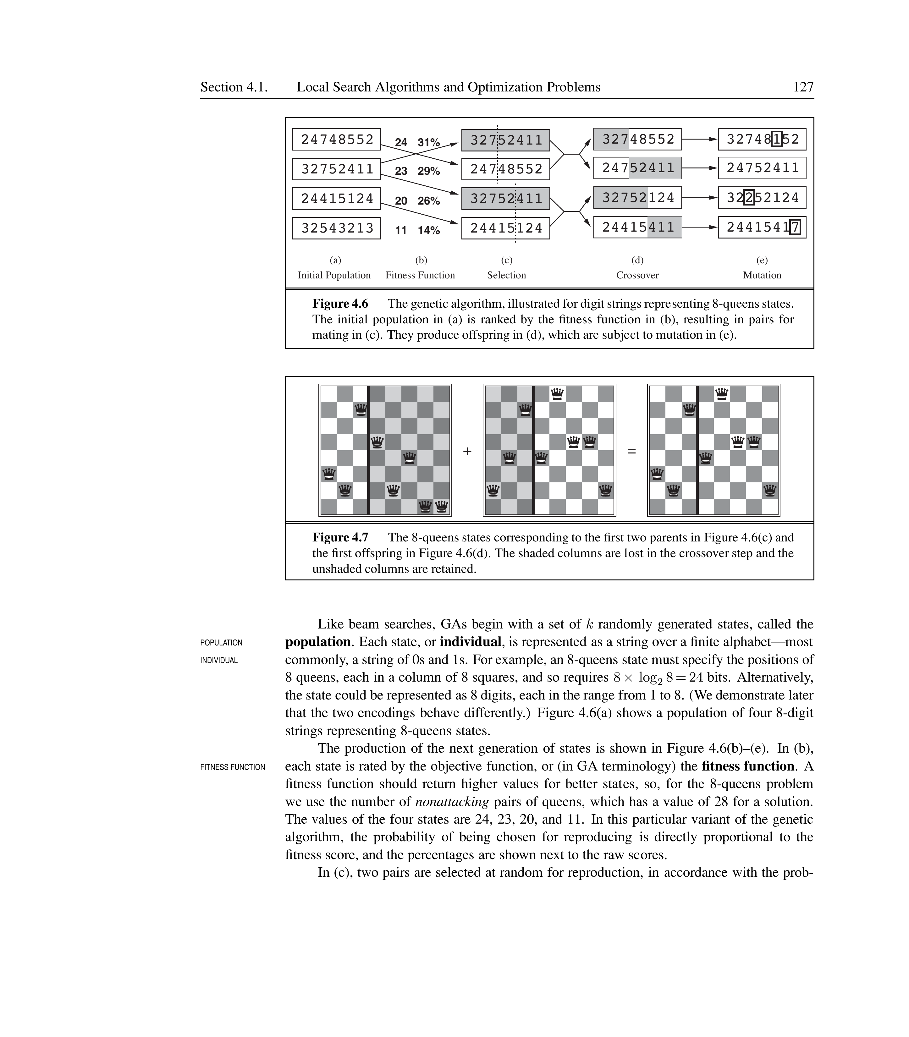
A variant of stochastic beam search in which successor states are generated by combining two parent states rather than modifying a single state. It maintains a population of individuals (states), each represented as a string over a finite alphabet. A fitness function rates the quality of each individual.
Key operations:
Selection: Choose individuals to reproduce, with probability proportional to fitness.
Crossover: Combine two parent strings at a randomly chosen crossover point to create offspring.
Mutation: Alter each position with a small independent probability.
Schema: A substring pattern (e.g., 246*****) describing a subset of states. Schemata with above-average fitness grow in the population over time.
8-Queens GA Example
Population of 4 states: 24748552 (fitness 24), 32752411 (fitness 23), 24415124 (fitness 20), 32543213 (fitness 11). Selection probabilities: 31%, 29%, 26%, 14%. Crossover at position 3 and 5 produces offspring like 32748552 and 24752411. Mutation changes one digit in some offspring.

Local Search in Continuous Spaces
Continuous Optimization
Many real-world environments are continuous — states are defined by an $n$-dimensional vector of variables $\mathbf{x} = (x_1, x_2, \ldots, x_n)$. The objective function $f(\mathbf{x})$ must be optimized over this continuous space.
Figure: Taxonomy of continuous optimization methods.
Methods for continuous optimization:
Discretization: Move only by a fixed amount $\pm\delta$ in each coordinate. This gives a finite set of successors for each state.
Gradient descent (steepest ascent): Use the gradient $\nabla f$ to find the direction of steepest slope and update:
Gradient
The gradient $\nabla f$ is a vector of partial derivatives giving the magnitude and direction of the steepest slope. \(\nabla f = \left( \frac{\partial f}{\partial x_1}, \frac{\partial f}{\partial x_2}, \ldots, \frac{\partial f}{\partial x_n} \right)\)
Key concepts:
Step size ($\alpha$): If too small, too many steps are needed. If too large, the search may overshoot the maximum.
Empirical gradient: When the objective function is not differentiable, calculate gradient by evaluating response to small increments and decrements in each coordinate.
Line search: Extend the current gradient direction by repeatedly doubling $\alpha$ until $f$ starts to decrease again.
Newton–Raphson method: Uses the Hessian matrix of second derivatives for faster convergence:
Constrained Optimization
An optimization problem with hard constraints on variable values. Linear programming deals with linear constraints (forming a convex set) and a linear objective function. Convex optimization allows any convex constraint region and any convex objective function. Both are solvable in polynomial time.
Airport Siting Problem
Place three new airports anywhere in Romania to minimize the sum of squared distances from each city to its nearest airport. The state space is 6-dimensional: $(x_1, y_1, x_2, y_2, x_3, y_3)$. The objective function sums distances for cities assigned to each airport: \(f(x_1, y_1, x_2, y_2, x_3, y_3) = \sum_{i=1}^{3} \sum_{c \in C_i} \left[ (x_i - x_c)^2 + (y_i - y_c)^2 \right]\) where $C_i$ is the set of cities closest to airport $i$.
Searching with Nondeterministic Actions
Contingency Plan (Strategy)
When the environment is nondeterministic, the solution to a problem is not a fixed action sequence but a contingency plan (or strategy) that specifies what to do depending on what percepts are received. Solutions become trees rather than sequences.
The Erratic Vacuum World
In the erratic vacuum world, the Suck action is nondeterministic:
Applied to a dirty square: cleans the square and sometimes cleans dirt in an adjacent square.
Applied to a clean square: sometimes deposits dirt.
Instead of a single RESULT function, we use a RESULTS function that returns a set of possible outcome states.
Erratic Vacuum Contingency Plan
Starting in state 1 (both squares dirty, agent in left square): \([\text{Suck}, \text{if State} = 5 \text{ then } [\text{Right}, \text{Suck}] \text{ else } [\;]]\) This plan works for both possible outcomes of the Suck action.
AND–OR Search Trees
AND–OR Search Tree
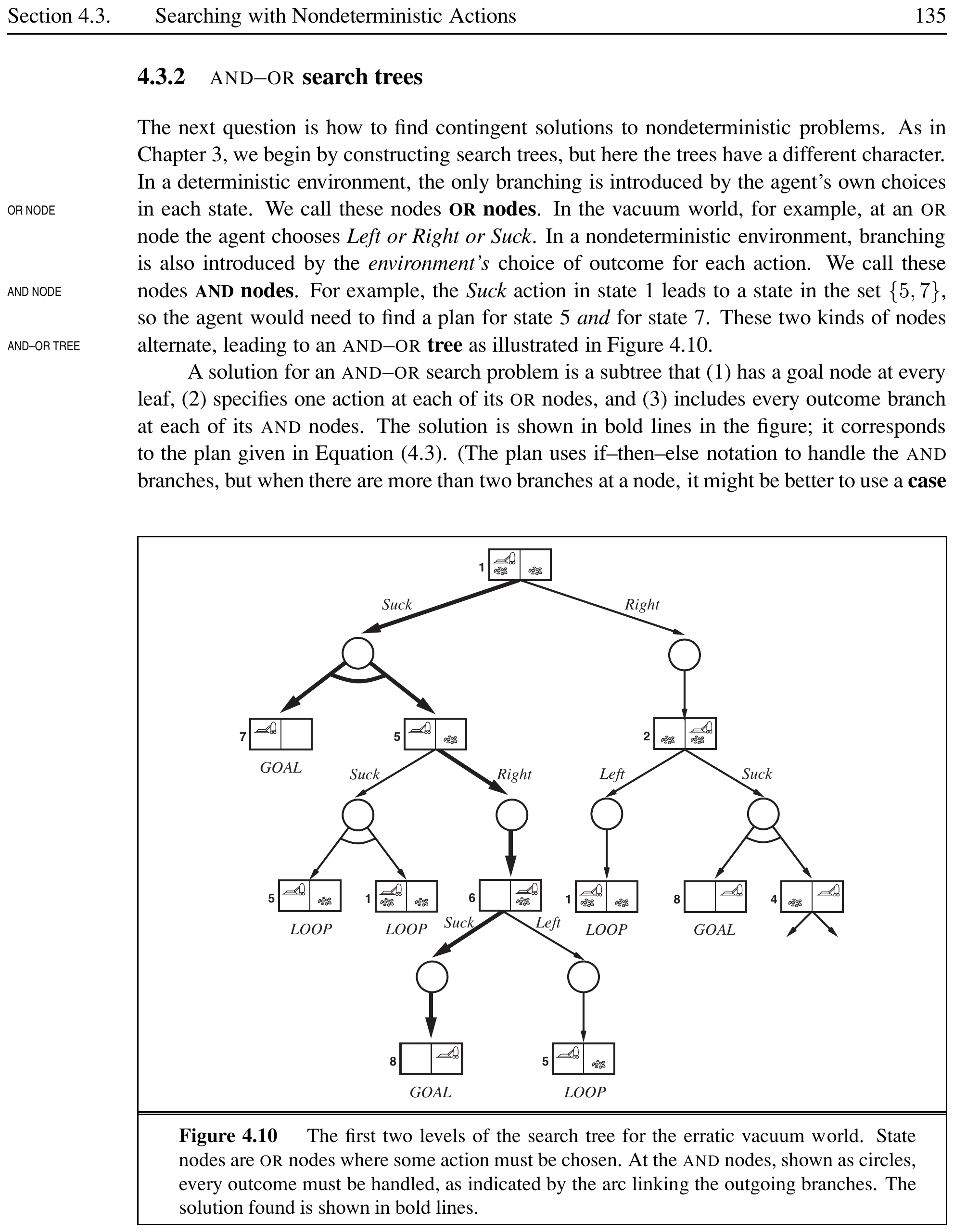
A search tree for nondeterministic environments with two types of nodes:
OR nodes: The agent chooses an action (branching by the agent’s choice).
AND nodes: The environment chooses the outcome (branching by the environment’s choice). Every outcome branch must be handled.
A solution is a subtree that (1) has a goal node at every leaf, (2) specifies one action at each OR node, and (3) includes every outcome branch at each AND node.
Cyclic Solutions
In the slippery vacuum world, movement actions sometimes fail. There are no acyclic solutions, but a cyclic solution exists: keep trying Right until it works.
Cyclic Plan (Slippery Vacuum World)
\([\text{Suck}, L_1: \text{Right}, \text{if State} = 5 \text{ then } L_1 \text{ else Suck}]\) This plan loops until the action succeeds, then proceeds.
Searching with Partial Observations
Belief State
The belief state represents the set of possible physical states the agent might be in, given the sequence of actions and percepts up to that point. In a partially observable environment, the agent uses its belief state to reason about what to do next.

Searching with No Observation (Sensorless Search)
Sensorless (Conformant) Problem
A problem where the agent receives no percepts at all. Despite having no sensors, the agent can often solve problems by using actions to reduce uncertainty. Searching happens in the space of belief states rather than physical states.
Key insight: The agent can coerce the world into a goal state by finding an action sequence that works regardless of the actual initial state.
Sensorless Vacuum World
Initial belief state: ${1, 2, 3, 4, 5, 6, 7, 8}$ (complete ignorance). The action sequence [Right, Suck, Left, Suck] is guaranteed to reach the goal state 7 no matter what the start state. Each action reduces uncertainty about the current state.
Prediction: The process of generating the new belief state after an action:
\[b' = \text{PREDICT}(b, a) = \{ s' : s' \in \text{RESULTS}(s, a) \text{ and } s \in b \}\]Searching with Observations
For general partially observable problems, transitions happen in three stages:
Prediction: Given action $a$ in belief state $b$, compute $\hat{b} = \text{PREDICT}(b, a)$.
Observation prediction: Determine the set of possible percepts: \(\text{POSSIBLE-PERCEPTS}(\hat{b}) = \{ o : o = \text{PERCEPT}(s) \text{ and } s \in \hat{b} \}\)
Update: For each possible percept $o$, compute the new belief state: \(b_o = \{ s : o = \text{PERCEPT}(s) \text{ and } s \in \hat{b} \}\)
Recursive State Estimation
Maintaining the belief state over time is called monitoring, filtering, or state estimation. The new belief state is computed from the previous one using: \(b' = \text{UPDATE}(\text{PREDICT}(b, a), o)\) This is a recursive state estimator — it does not re-examine the entire percept sequence.
Robot Localization
A robot with sonar sensors in a maze receives percept NSW (obstacles to north, west, south). After update, the belief state shrinks to 4 possible locations. After a Move action and a second percept NS, the belief state collapses to a single location. The robot has localized itself.
Online Search Agents and Unknown Environments
Offline vs. Online Search
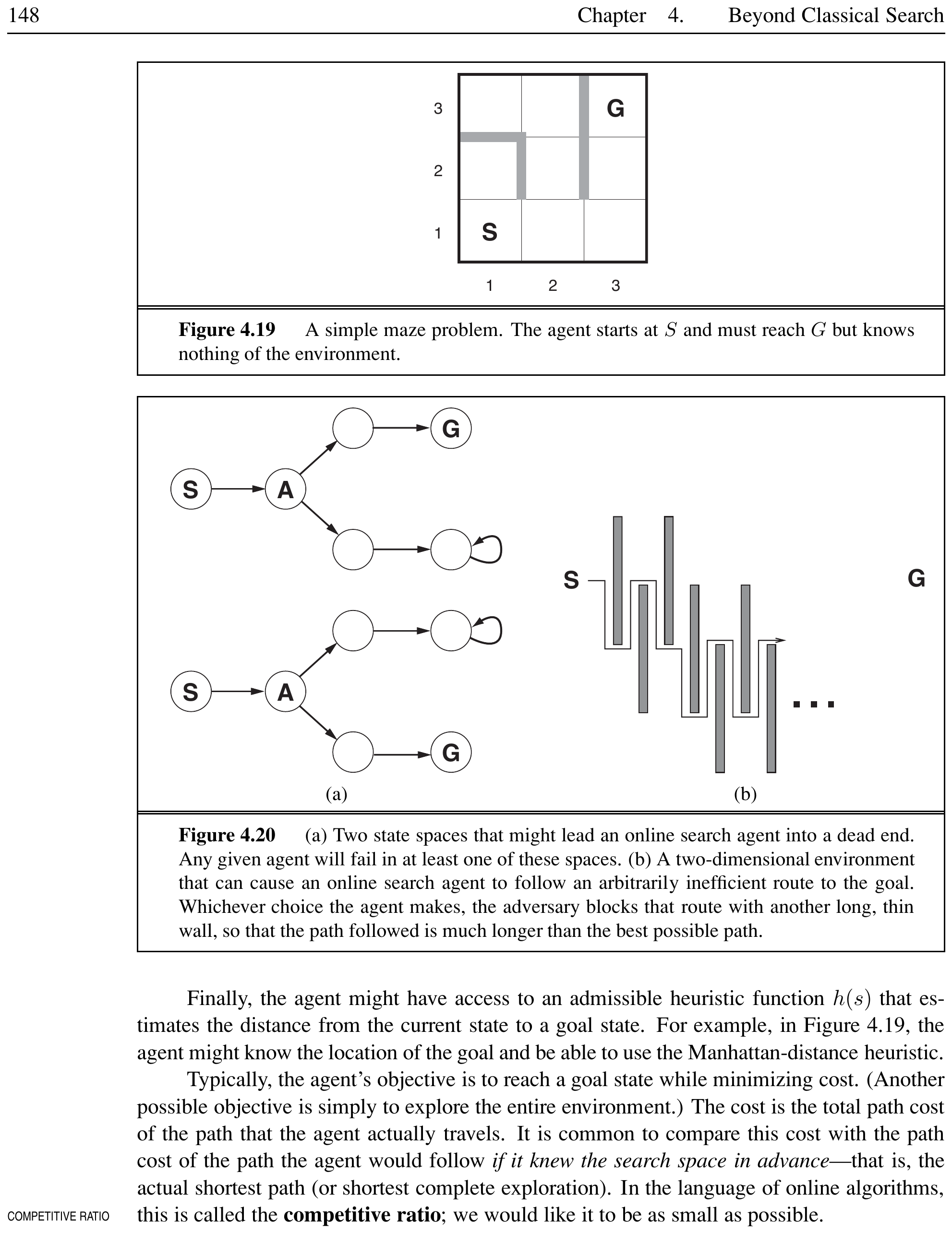
Offline search computes a complete solution before executing any actions. Online search interleaves computation and action: the agent acts, observes the environment, and computes the next action. Online search is necessary for unknown environments where the agent does not know what states exist or what its actions do — it faces an exploration problem.
Online Search Problems
The agent knows only: ACTIONS(s), step-cost function $c(s, a, s’)$, and GOAL-TEST(s). It cannot determine RESULT(s, a) without actually being in $s$ and doing $a$.
Competitive Ratio
The ratio of the cost of the path the agent actually travels to the cost of the optimal path the agent would follow if it knew the search space in advance. \(\text{Competitive Ratio} = \frac{\text{Actual Path Cost}}{\text{Optimal Path Cost}}\)
Dead End and Safely Explorability
A dead end is a state from which no goal state is reachable. A state space is safely explorable if some goal state is reachable from every reachable state. Reversible action spaces (e.g., mazes, 8-puzzle) are safely explorable.
Online Search Agents
Online DFS agent: Uses depth-first exploration. Stores results in a table RESULT[s, a]. Backtracks physically to the previous state. Works only in reversible state spaces.
LRTA* (Learning Real-Time A*)
An online local search agent that stores a current best estimate $H(s)$ of the cost to reach the goal from each visited state. It updates $H(s)$ based on experience: \(H[s] \leftarrow \min_{b \in \text{ACTIONS}(s)} \text{LRTA*-COST}(s, b, \text{result}[s, b], H)\) where $\text{LRTA*-COST}(s, a, s’, H) = c(s, a, s’) + H[s’]$ for known outcomes, or $h(s)$ for untried actions.
Optimism Under Uncertainty
LRTA* assumes that actions not yet tried lead immediately to the goal with the least possible cost $h(s)$. This optimism under uncertainty encourages the agent to explore new, potentially promising paths.
Random walk: Selects randomly from available actions. Eventually finds a goal in any finite space, but can be exponentially slow in some environments.
LRTA* Example
In a one-dimensional state space, the agent starts with heuristic estimates. When stuck in a local minimum, it updates $H$ values by observing the actual costs of neighboring states. Over several iterations, the local minimum is “flattened out” and the agent escapes to the right toward the goal. LRTA* is guaranteed to find a goal in any finite, safely explorable environment.
Learning in Online Search
Online agents learn a map of the environment by recording action outcomes. LRTA* acquires more accurate cost estimates through local updating rules. These updates eventually converge to exact values, making pure hill climbing an optimal strategy.
Exam-Style Question
Explain the difference between local search and systematic search. Why is local search useful for optimization problems? Discuss the problem of local maxima and how random-restart hill climbing addresses it.
Solution
Systematic search (BFS, DFS, A*) keeps multiple paths in memory and explores the state space methodically. Local search operates on a single current state, moving only to neighbors. It uses very little memory and works well in large or continuous spaces. However, it can get stuck in local maxima. Random-restart hill climbing addresses this by running multiple hill-climbing searches from random initial states, making it complete with probability approaching 1.
| Algorithm | Memory | Completeness | Key Feature | ||
|---|---|---|---|---|---|
| Hill Climbing | $O(1)$ | No | Moves to best neighbor | ||
| Random-Restart HC | $O(1)$ | Yes (prob. 1) | Multiple random starts | ||
| Simulated Annealing | $O(1)$ | Yes (with slow schedule) | Probabilistic downhill moves | ||
| Local Beam Search | $O(k)$ | No | Tracks $k$ states in parallel | ||
| Genetic Algorithm | $O(N)$ | No | Crossover + mutation | ||
| LRTA* | $O( | S | )$ | Yes (finite safe spaces) | Learns cost estimates |
Comparison of Local Search Algorithms