Constraint Satisfaction Problems
CSPs, constraint propagation, backtracking search, and problem structure.
Constraint Satisfaction Problems
Defining Constraint Satisfaction Problems
Constraint Satisfaction Problem
A constraint satisfaction problem (CSP) consists of three components:
X — a set of variables, ${X_1, X_2, \dots, X_n}$.
D — a set of domains, ${D_1, D_2, \dots, D_n}$, one for each variable.
C — a set of constraints that specify allowable combinations of values.
Each domain $D_i$ is the set of allowable values for variable $X_i$. Each constraint $C_i$ is a pair $\langle scope, rel \rangle$, where $scope$ is a tuple of variables and $rel$ is a relation defining the values those variables may take.

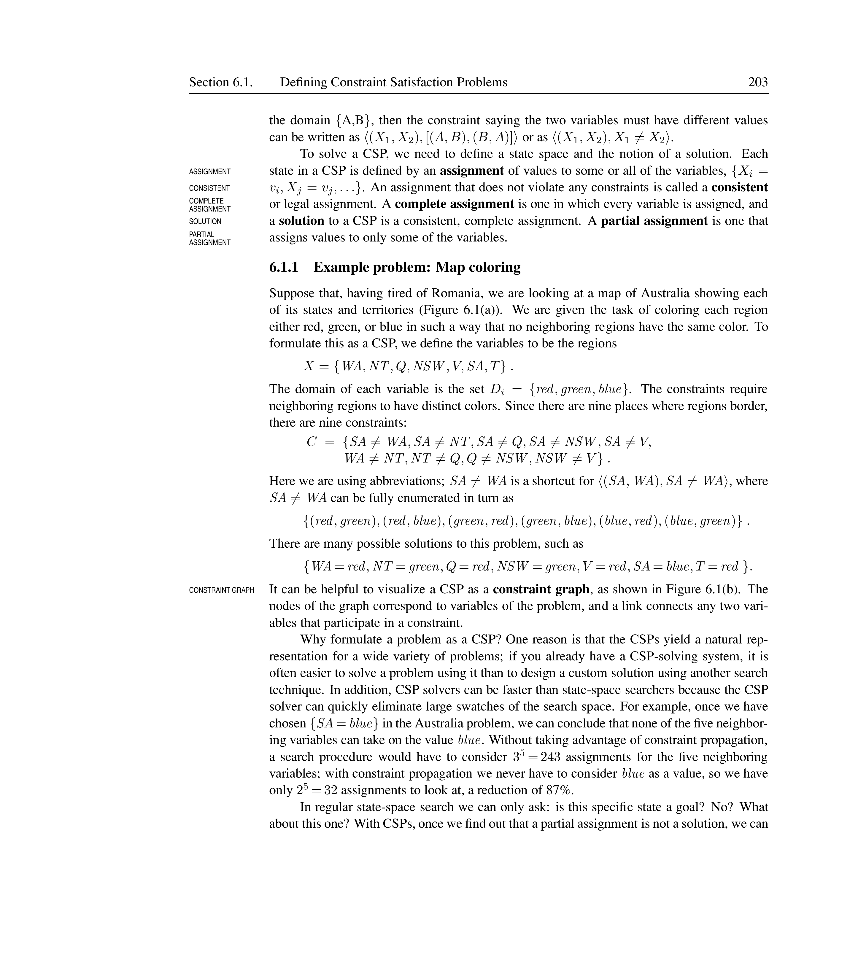
An assignment maps variables to values: ${X_i = v_i, X_j = v_j, \dots}$. A consistent (or legal) assignment does not violate any constraints. A complete assignment assigns every variable. A solution to a CSP is a consistent, complete assignment. A partial assignment assigns only some variables.
Map Coloring
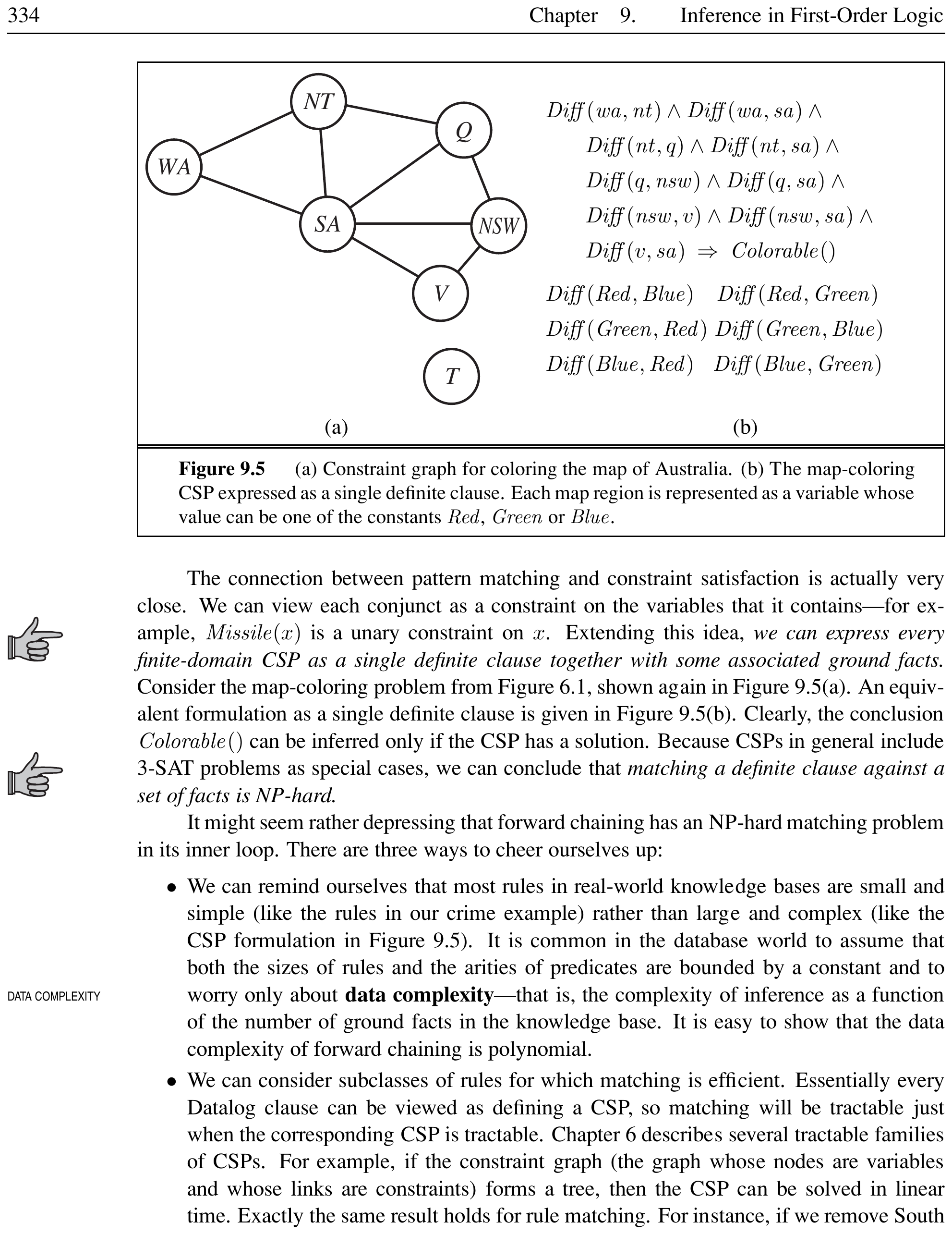
Coloring the states of Australia with three colors (red, green, blue) such that no neighboring regions share a color:
Variables: $X = {WA, NT, Q, NSW, V, SA, T}$.
Domains: Each $D_i = {red, green, blue}$.
Constraints: $SA \neq WA$, $SA \neq NT$, $SA \neq Q$, $SA \neq NSW$, $SA \neq V$, $WA \neq NT$, $NT \neq Q$, $Q \neq NSW$, $NSW \neq V$.
A solution: ${WA = red, NT = green, Q = red, NSW = green, V = red, SA = blue, T = red}$.
A CSP can be visualized as a constraint graph, where nodes represent variables and edges connect variables that share a constraint.
Variations on the CSP Formalism
Discrete domains.
A finite domain, e.g., ${red, green, blue}$ for map coloring. An infinite discrete domain, e.g., the set of integers for job scheduling start times.
Continuous domains.
Common in operations research, e.g., scheduling Hubble Space Telescope observations with continuous-valued start and finish times. Linear programming is the best-known category.
Constraint types.
Unary constraint: restricts a single variable, e.g., $SA \neq green$.
Binary constraint: relates two variables, e.g., $SA \neq NSW$.
Global constraint: involves an arbitrary number of variables, e.g., $Alldiff(F, T, U, W, R, O)$ in cryptarithmetic.
Preference constraints
indicate which solutions are preferred (soft constraints). These can be encoded as costs, leading to a constraint optimization problem (COP).
Job-Shop Scheduling
Scheduling car assembly with 15 tasks (install axles, affix wheels, tighten nuts, attach hubcaps, inspect):
Variables: ${Axle_F, Axle_B, Wheel_{RF}, \dots, Inspect}$.
Domains: $D_i = {1, 2, \dots, 27}$ (start times in minutes).
Precedence constraints: $Axle_F + 10 \leq Wheel_{RF}$, $Wheel_{RF} + 1 \leq Nuts_{RF}$, etc.
Disjunctive constraint: $(Axle_F + 10 \leq Axle_B)$ or $(Axle_B + 10 \leq Axle_F)$.
Inspection: $X + d_X \leq Inspect$ for all $X \neq Inspect$.
Constraint Propagation: Inference in CSPs
Constraint Propagation
Constraint propagation uses the constraints to reduce the number of legal values for a variable, which in turn reduces the legal values for other variables. The key idea is local consistency: ensuring that each part of the constraint graph satisfies a local condition, causing inconsistent values to be eliminated throughout the graph.
Node Consistency
Node Consistency
A variable is node-consistent if all values in its domain satisfy its unary constraints. A network is node-consistent if every variable is node-consistent.
Node Consistency in Australia
If $SA$ cannot be green (a unary constraint), we remove green from $D_{SA}$, leaving ${red, blue}$. This makes $SA$ node-consistent.
Arc Consistency
Arc Consistency
$X_i$ is arc-consistent with respect to $X_j$ if for every value $v \in D_i$ there exists some value $w \in D_j$ satisfying the binary constraint on the arc $(X_i, X_j)$. A network is arc-consistent if every variable is arc-consistent with every other.
Arc Consistency with $Y = X^2$
Let $X$ and $Y$ have domain ${0, 1, 2, 3, 4}$, with constraint $Y = X^2$: \(\langle (X, Y), \{(0,0), (1,1), (2,4), (3,9)\} \rangle\)
Make $X$ arc-consistent wrt $Y$: reduce $D_X$ to ${0, 1, 2, 3}$.
Make $Y$ arc-consistent wrt $X$: reduce $D_Y$ to ${0, 1, 4, 9}$.
Now the CSP is arc-consistent.

The AC-3 algorithm maintains a queue of arcs. When $D_i$ is revised, all arcs $(X_k, X_i)$ for neighbors $X_k$ are added to the queue. AC-3 runs in $O(c d^3)$ time for $n$ variables, domain size at most $d$, and $c$ binary constraints.
AC-3 on Sudoku
In a Sudoku puzzle with Alldiff constraints expanded to binary constraints:
Variable $E6$ (center box): removing 2, 8, 1, 7 from box constraints, then 5, 6, 2, 8, 9, 3 from column constraints. Domain reduces to ${4}$.
AC-3 can solve the entire easiest Sudoku puzzles without search.
Path Consistency
Path Consistency
A two-variable set ${X_i, X_j}$ is path-consistent with respect to a third variable $X_m$ if for every consistent assignment ${X_i = a, X_j = b}$, there exists an assignment to $X_m$ that satisfies the constraints on ${X_i, X_m}$ and ${X_m, X_j}$.
Path Consistency with Two Colors
Coloring Australia with only two colors (red, blue). Arc consistency does nothing (every value has a valid neighbor). But path consistency of ${WA, SA}$ with respect to $NT$ reveals that no valid assignment exists — proving the problem unsolvable.
$k$-Consistency
$k$-Consistency
A CSP is $k$-consistent if for any set of $k-1$ variables and any consistent assignment to those variables, a consistent value can always be assigned to any $k$th variable.
1-consistency = node consistency.
2-consistency = arc consistency.
3-consistency = path consistency (for binary networks).
A CSP is strongly $k$-consistent if it is $k$-consistent and also $(k-1)$-consistent, $(k-2)$-consistent, …, 1-consistent.
Strong $n$-Consistency
A strongly $n$-consistent CSP with $n$ variables can be solved in $O(n^2 d)$ time: assign $X_1$, then $X_2$ (guaranteed by $2$-consistency), then $X_3$ (guaranteed by $3$-consistency), and so on. However, achieving $n$-consistency is exponential in $n$, so this is rarely practical.
Global Constraints and Bounds Propagation
Alldiff Constraint
The Alldiff constraint requires all variables in its scope to have distinct values. If $m$ variables have $n$ possible distinct values and $m > n$, the constraint cannot be satisfied.
Bounds Consistency
A CSP is bounds consistent if for every variable $X$, and for both the lower-bound and upper-bound values of $X$, there exists some value of $Y$ that satisfies the constraint between $X$ and $Y$ for every variable $Y$.
Bounds Propagation for Two Flights
Two flights have capacities $D_1 = [0, 165]$, $D_2 = [0, 385]$ and must carry 420 people total ($F_1 + F_2 = 420$). Bounds propagation reduces domains to $D_1 = [35, 165]$, $D_2 = [255, 385]$.
Backtracking Search for CSPs
Backtracking Search
Backtracking search is a depth-first search that assigns values to one variable at a time and backtracks when a variable has no legal values left. It exploits commutativity of CSPs: the order of assignments does not affect the outcome, so we only consider one variable at each node.
Commutativity in CSP Search
Without commutativity: for $n$ variables with domain size $d$, the top branching factor is $nd$, yielding $n! \cdot d^n$ leaves. With commutativity (assigning one variable at a time), only $d^n$ leaves remain. For $n=7, d=3$ (Australia): $7! \cdot 3^7 \approx 2.2 \times 10^7$ vs. $3^7 = 2187$ leaves.
Variable and Value Ordering
MRV Heuristic
The minimum-remaining-values (MRV) heuristic chooses the unassigned variable with the fewest legal values. Also called the “most constrained variable” or “fail-first” heuristic.
MRV in Australia
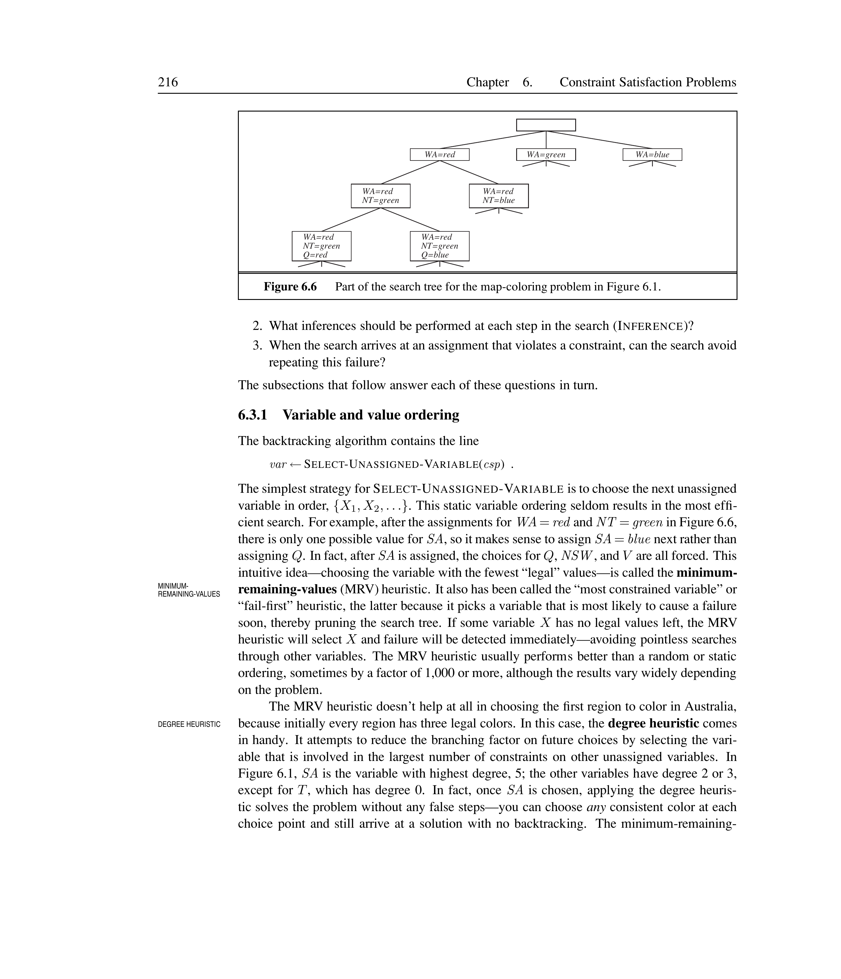
After $WA=red$ and $NT=green$, $SA$ has only 1 legal value (blue). MRV selects $SA$ next rather than $Q$, immediately forcing the rest of the solution.
Degree Heuristic
The degree heuristic selects the variable involved in the largest number of constraints on other unassigned variables. Useful as a tie-breaker for MRV.
Degree in Australia
Initially all variables have 3 colors, so MRV cannot decide. The degree heuristic picks $SA$ (degree 5) over $WA, NT, Q$ (degree 2–3), eliminating the need for backtracking.
Least-Constraining-Value Heuristic
The least-constraining-value (LCV) heuristic prefers the value that rules out the fewest choices for neighboring variables. This is a “fail-last” strategy.
LCV for Queensland
Given $WA=red$ and $NT=green$, $Q$ can be red or blue. Blue is a bad choice — it eliminates the last legal value for $SA$. LCV therefore prefers red, leaving maximum flexibility for $SA$.
Interleaving Search and Inference
Forward Checking
Forward checking establishes arc consistency for each newly assigned variable: whenever $X$ is assigned a value, delete from each unassigned neighbor $Y$ any value inconsistent with $X$.
MAC (Maintaining Arc Consistency)
MAC applies AC-3 after each variable assignment, starting with arcs from the assigned variable to its unassigned neighbors. MAC is strictly more powerful than forward checking because it propagates changes recursively.
Forward Checking on Australia
Assign $WA = red$: delete red from $NT$ and $SA$.
Assign $Q = green$: delete green from $NT$, $SA$, $NSW$.
Assign $V = blue$: delete blue from $NSW$ and $SA$ — $SA$ domain is now empty, backtrack immediately.
Intelligent Backtracking
Chronological Backtracking
Chronological backtracking reverts to the most recently assigned variable when a dead end is reached. This can be inefficient because it may backtrack to irrelevant variables.
Chronological Backtracking Failure
With ordering $Q, NSW, V, T, SA, WA, NT$, suppose we reach $SA$ after assigning $Q=red, NSW=green, V=blue, T=red$ and find no legal value for $SA$. Chronological backtracking re-colors $T$, but Tasmania is irrelevant to $SA$’s failure.
Conflict-Directed Backjumping
Conflict-directed backjumping maintains a conflict set for each variable (the set of prior assignments that conflict with its values). When a variable has no legal values, backjump to the most recent variable in its conflict set, merging conflict sets.
Backjumping over Tasmania
Continuing the previous example: $SA$’s conflict set is ${Q, NSW, V}$ (not $T$). Backjumping goes directly back to $V$, skipping the irrelevant $T$ entirely.
Constraint Learning
Constraint learning records no-goods — minimal sets of variable assignments that cause inconsistency — preventing the search from repeating the same failure. This is one of the most important techniques in modern CSP solvers.
No-Good Recording
If ${Q=red, NSW=green, V=blue}$ causes $SA$ to have no legal values, the no-good ${Q=red, NSW=green, V=blue}$ is recorded. Any future branch containing this triple is pruned immediately.
Local Search for CSPs
Min-Conflicts Heuristic
Min-conflicts is a local search algorithm for CSPs using a complete-state formulation:
Start with a random assignment to every variable.
At each step, choose a randomly selected conflicted variable.
Assign it the value that minimizes the number of violated constraints.
Min-Conflicts on $n$-Queens
The min-conflicts heuristic is surprisingly effective: on the $n$-queens problem, run time is roughly independent of problem size. It can solve the million-queens problem in about 50 steps on average. Solutions are densely distributed in the state space for $n$-queens.
Constraint Weighting
Constraint Weighting
Constraint weighting assigns a numeric weight $W_i$ to each constraint (initially 1). At each step, the algorithm chooses a variable/value pair minimizing the total weight of violated constraints, then increments weights of currently violated constraints.
Constraint weighting adds topography to plateaux and focuses search on difficult constraints over time.
Constraint Weighting in Map Coloring
Initially all $W_i = 1$. The algorithm picks a coloring and increments weights of violated edges. Over multiple runs, the edge $SA$–$NT$ (which is hard to satisfy) accumulates a high weight, guiding future assignments to respect it earlier.
Applications
Local search for CSPs is particularly effective for scheduling problems. For example, min-conflicts has been used to schedule Hubble Space Telescope observations, reducing scheduling time from three weeks to 10 minutes. It also handles online problem changes well — repairing a schedule when conditions change, rather than rebuilding from scratch.
The Structure of Problems
Tree-Structured CSP
A constraint graph is a tree if any two variables are connected by only one path. Tree-structured CSPs can be solved in linear time using directed arc consistency (DAC).
Solving Tree-Structured CSPs
Choose any variable as root and perform a topological sort.
Make the graph directed arc-consistent: for each variable $X_i$, ensure arc consistency with each $X_j$ for $j > i$.
Assign variables in order; each assignment has a guaranteed valid choice for the next variable.
Solving a Tree-Structured CSP
Given variables $A, B, C, D$ in a chain $A-B-C-D$ with domain ${0,1}$ and constraints $A \neq B$, $B \neq C$, $C \neq D$:
Topological sort: $A, B, C, D$.
DAC from leaves to root: enforce $A \to B$, $B \to C$, $C \to D$.
Assign $A=0$ (arbitrary), then $B=1$, $C=0$, $D=1$ without backtracking.
Independent Subproblems
Connected Components
If the constraint graph has multiple connected components (disjoint subgraphs with no edges between them), each component forms an independent subproblem. The solution to the overall CSP is the union of the solutions to each component.
Splitting a CSP into independent subproblems dramatically reduces the search complexity. If a CSP with $n$ variables and domain size $d$ is split into $m$ components of size $n_1, n_2, \dots, n_m$, the total complexity is:
\[O(d^{n_1} + d^{n_2} + \dots + d^{n_m}) \ll O(d^n)\]Independent Subproblems in Australia
The Australia constraint graph has two connected components: the mainland (WA, NT, Q, SA, NSW, V) and Tasmania (T). Since $T$ is only adjacent to $NSW$, we solve each separately. Complexity drops from $O(3^7) = 2187$ to $O(3^6 + 3^1) = 732$ — a $3\times$ reduction.
Cycle Cutset
Cycle Cutset
A cycle cutset is a subset $S$ of variables whose removal makes the constraint graph a tree. The approach of cutset conditioning assigns values to $S$, then solves the remaining tree-structured CSP.
| where $c = | S | $. Finding the smallest cycle cutset is NP-hard, but good approximation algorithms exist. |
Cycle Cutset on Australia
The Australia graph has cycles (e.g., WA–NT–SA–WA). Choosing $S = {SA}$ breaks all cycles: removing $SA$ leaves a tree (WA, NT, Q, NSW, V, T). Cutset conditioning assigns $SA = red$ (or $blue$), then solves the remaining tree in $O((n-1)d^2)$. Total: $O(d \cdot (n-1)d^2)$.
Tree Decomposition
Tree Decomposition
A tree decomposition partitions the constraint graph into connected subproblems (clusters) arranged in a tree. Each subproblem is solved independently, and solutions are combined via shared variables.
Three requirements:
Every variable appears in at least one subproblem.
If two variables share a constraint, they appear together in at least one subproblem.
If a variable appears in two subproblems, it must appear in every subproblem along the path connecting them.
Tree Width
The tree width of a tree decomposition is one less than the size of the largest subproblem. The tree width of a graph is the minimum tree width over all decompositions. If tree width is $w$, the CSP can be solved in $O(n d^{w+1})$ time.
Tree Decomposition of Australia
The Australia map can be decomposed into 5 subproblems:
Subproblem 1: ${WA, SA, NT}$ — 3 regions.
Subproblem 2: ${SA, NT, Q}$ — shares $SA$ and $NT$ with subproblem 1.
Subproblem 3: ${SA, Q, NSW}$.
Subproblem 4: ${SA, NSW, V}$.
Subproblem 5: ${NSW, T}$.
Each subproblem is solved independently; solutions must agree on shared variables.
Symmetry Breaking
Value Symmetry
Value symmetry occurs when permuting the values in a solution yields another solution. A symmetry-breaking constraint imposes an ordering to eliminate symmetric solutions, reducing the search space.
Breaking Value Symmetry in Australia
With 3 colors (red, green, blue), the 3! = 6 solutions are just color renamings of the same structure. Adding $NT < SA < WA$ alphabetically (e.g., $NT = red$, $SA = green$, $WA = blue$) forces a canonical ordering and prunes 5 symmetric solutions.
Optimization Problems
Constraint Optimization Problem
A constraint optimization problem (COP) extends CSPs with preference constraints that assign costs to variable assignments. The goal is to find a solution that minimizes (or maximizes) an objective function while satisfying all absolute constraints.
Class Scheduling with Preferences
Absolute constraints: no professor teaches two classes at the same time.
Preference constraints: Prof. R prefers morning classes (cost 1) over afternoon (cost 2).
Objective: minimize total preference cost while satisfying all absolute constraints.
COPs can be solved with:
Branch-and-bound search (pruning branches whose partial cost exceeds the best known solution).
Local search with an objective function (hill climbing, simulated annealing).
Linear programming for continuous-domain COPs with linear constraints.
Linear Programming
A linear programming problem is a COP with continuous variables, linear constraints (equalities or inequalities), and a linear objective function. It can be solved in polynomial time using algorithms such as the simplex method or interior-point methods.
Production Planning as LP
A factory produces chairs ($x_1$) and tables ($x_2$). Profit: $5x_1 + 8x_2$. Constraints: $2x_1 + 3x_2 \leq 100$ (wood), $x_1 + 2x_2 \leq 60$ (labor), $x_1, x_2 \geq 0$. The simplex method finds the optimal production mix at the intersection of constraints.
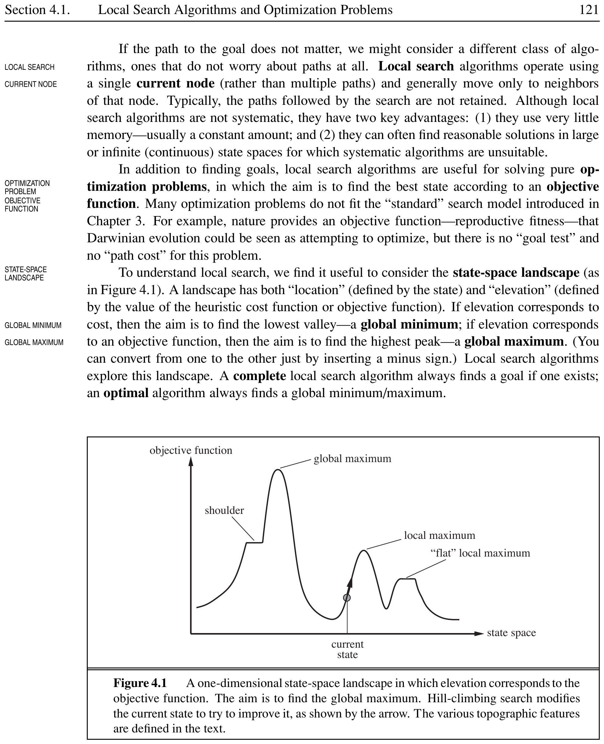
Summary
CSPs represent states as variable/value pairs and solutions as consistent complete assignments satisfying all constraints.
Inference techniques (node, arc, path, $k$-consistency) propagate constraints to reduce domains.
Backtracking search with MRV, degree, LCV heuristics and forward checking/MAC is the standard systematic approach.
Min-conflicts local search is surprisingly effective, especially for $n$-queens and scheduling problems.
Tree-structured CSPs are solvable in linear time; cycle cutset and tree decomposition methods handle more general structures.
Constraint optimization problems extend CSPs with preference constraints and an objective function.