Matlab Signal Onramp course notes - Part 2: Data Import & Signal Analyzer

Earthquake Example

In this series, we analyze seismic waves from the massive 2004 Sumatra earthquake. The vibrations traveled across the Earth and were recorded by three seismic stations in Alaska: HARP, PAX, and WANC.

The Workflow

1. Import the signals into MATLAB.
2. Preprocess to prepare for analysis.
3. Analyze in the time and frequency domains.
4. Filter to isolate specific frequency content.
5. Extract Information or deploy the algorithm.

---

Importing Signals

Seismic stations record vertical displacement. We can use readmatrix for simple numeric data or readtimetable when time information is crucial.

% Importing raw data
harp = readmatrix("harp.csv");

% Importing as a timetable with a 50 Hz sample rate
tbl = readtimetable("harp.csv", SampleRate=50);
plot(tbl, "Var1")

---

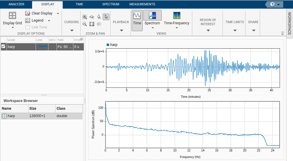
Signal Analyzer App

The Signal Analyzer app is a powerful interactive tool for inspecting, comparing, and preprocessing signals.

• Importing: Drag signals from the Workspace Browser.
• Time Values: Specify sample rate or time vectors.
• Spectrum View: Toggle the power spectrum to see frequency content.
• Panner: Zoom into specific time regions.

Viewing the Power Spectrum

The power spectrum shows the intensity of different frequencies. For the HARP signal, we see a peak around 0.05 Hz, corresponding to a wave every 20 seconds—the primary surface waves of the earthquake.

---

Comparing Multiple Signals

The three stations used different hardware, leading to different characteristics:

• HARP: Uniform 50 Hz sampling.
• PAX: Non-uniform sampling (imperfect hardware).
• WANC: Uniform 100 Hz sampling (faster rate).

By importing all three into the Signal Analyzer, we can compare their frequency content side-by-side.

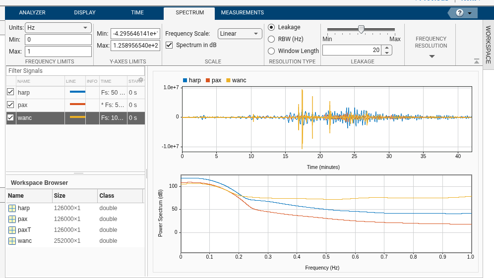
While they share low-frequency content (0–0.2 Hz), their amplitudes and high-frequency noise vary significantly. In the next part, we’ll use preprocessing to align these signals for a better comparison.