Matlab Image Processing Onramp: Preprocessing and Postprocessing

Preprocessing and Postprocessing Techniques

Improve Segmentation

Receipt Identification Workflow workflow with steps 2 and 4 highlighted: Preprocess and Postprocess Preprocess and Postprocess to Improve Segmentation

Segmentation can be improved in two ways: by preprocessing the image before binarizing and by postprocessing the binary image itself.

You’ve already done some preprocessing by converting each image to grayscale and adjusting the contrast. In the next few activities, you use three additional preprocessing and postprocessing techniques.

Noise Removal Figure 1: Smooth pixel intensity values to reduce the impact of variation on binarization.

Background Isolation and Subtraction Figure 2: Isolate and remove the background of an image before binarizing.

Binary Morphology Figure 3: Emphasize particular patterns or shapes in a binary image.

Filter Noise

(1/2) Spatial Filtering

Spatial Filtering Spatial filtering is a powerful technique to enhance images or their features. Noisy images can contain individual pixels with noticeably different intensity values than their neighbors. An averaging filter can smooth out these differences by replacing each pixel’s value with the average of itself and neighboring pixels. A filter is a matrix that acts as a mask, creating a window around a pixel to perform operations. Applying a filter involves performing operations like weighted averages on the window, resulting in a new filtered image. Different filters serve different purposes, such as blurring edges or removing noise. Sometimes no matter which threshold we pick, we can’t quite seem to get a good binary image. See these pesky specks? Well, they’re the result of having a noisy image. We can see many places in the original image where an individual pixel has a noticeably different intensity value than the pixels surrounding it.

You can smooth out these differences by using a technique called spatial filtering. Spatial filtering is a neighborhood operation where each pixel’s value is changed based on neighboring pixel values. How the pixel’s value changes depends on the filter.

So, what is a filter? Well, a filter is a matrix, and it acts like a mask. When you place the filter over part of an image, it creates a window or neighborhood around a pixel. To apply a filter, you perform some operation on that window. For example, a linear filter performs a weighted average. So, you multiply the values in the filter and the image and add the results. This gives you a single value that you can think of as the new filtered value for that pixel. Then move the filter over to the next pixel and repeat. Applying the filter to every pixel gives you a new filtered image.

Operations like this are sometimes called sliding window operations. Different filters have different purposes, determined by the values in the filter matrix. For example, this filter replaces each pixel with the average of itself and the eight pixels around it. It’s good for blurring edges and removing noise. Well, that sounds useful. In this next activity, you’ll learn how to create and apply this filter in MATLAB.

(2/2) Remove Noise from an Image

Image Noise

You can increase the light sensitivity of a digital camera sensor to improve the brightness of a picture taken in low light. Many modern digital cameras (including mobile phone cameras) automatically increase the ISO in dim light. However, this increase in sensitivity amplifies noise picked up by the sensor, leaving the image grainy (shown on the left).

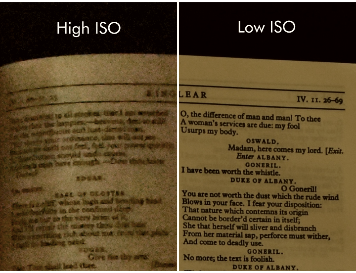Figure 4: Camera Sensor Noise

Images taken in low light often become noisy due to the increase in camera sensitivity required to capture the image. This noise can interfere with receipt identification by polluting regions in the binarized image.

To reduce the impact of this noise on the binary image, you can preprocess the image with an averaging filter.

Use the fspecial function to create an n-by-n averaging filter.

F = fspecial("average",n)

Task Create a 3-by-3 averaging filter and store the result in H.

H = fspecial("average", 3)

You can apply a filter F to an image I by using the imfilter function.

Ifltr = imfilter(I,F);

Task Apply the filter H to the grayscale image gs. Store the result in gssmooth.

gssmooth = imfilter(gs, H);

Now that you have filtered the image, you can binarize it. Did the filter reduce the amount of noise in the binary image? Task Create a binary image from gssmooth using imbinarize with the “adaptive” setting and “ForegroundPolarity” set to “dark”. Store the result in BWsmooth and display it.

BWsmooth = imbinarize(gssmooth, "adaptive", ...
    "ForegroundPolarity", "dark" ...
);
imshow(BWsmooth)

If you look closely, you can see that filtering introduced a small, unwanted dark outline to parts of the binary image border. The reason is that the default setting of imfilter sets pixels outside the image to zero.

To adjust this behavior, use the “replicate” option.

Ifltr = imfilter(I,F,"replicate");

Instead of zeros, the “replicate” option uses pixel intensity values on the image border for pixels outside the image. Task Apply the filter H to the grayscale image gs as you did in Task 2, but use the “replicate” option. Store the filtered image in gssmooth.

gssmooth = imfilter(gs, H, "replicate");
imshow(gssmooth)

Because you used the “replicate” option, the filtered image should no longer contain an artificial border. Use the imbinarize function to create a new binary image. Has the border been removed? Task Binarize gssmooth as you did in Task 3, and store the result in BWsmooth. Display BWsmooth.

BWsmooth = imbinarize(gssmooth, "adaptive", ...
    "ForegroundPolarity", "dark");
imshow(BWsmooth);

Compute the row sums for both the original and smoothed binary images, BW and BWsmooth. Plot these signals together on the same axes using the hold on and hold off commands.

Do you notice any improvements in the row sum of BWsmooth when compared to the row sum of BW?

Background Subtraction

(1/3) Isolate the Image Background

Isolate the Image Background

Receipt images that have a busy background are more difficult to classify because artifacts pollute the row sum. To mitigate this issue, you can isolate the background and then remove it by subtraction.

In a receipt image, the background is anything that is not text, so isolating the background can be interpreted as removing the text. One way to remove text from an image is to use morphological operations.

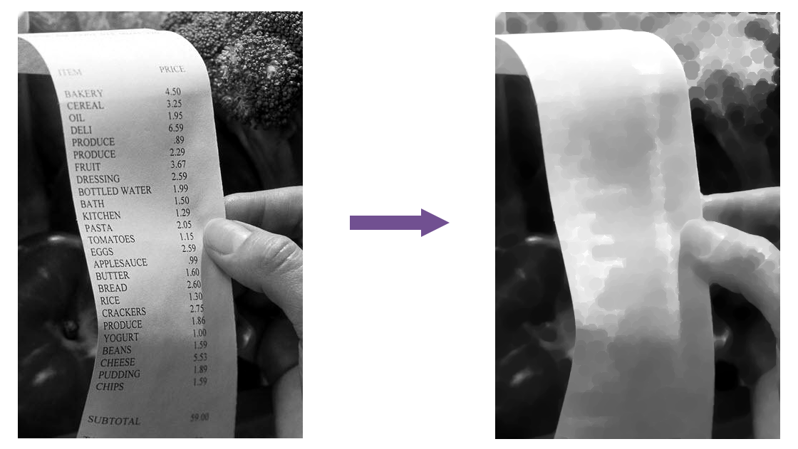Figure 5: A grayscale image of a receipt next to the same receipt with isolated background. A morphological closing operation emphasizes the bright paper and removes the dark text.

(2/3) Morphological Operations

Morphological Operations Morphological operations are sliding window operations that use a structuring element to determine which neighboring pixels to include for each calculation. You can change the size and shape of the structuring element to affect the output of morphological operations. Dilation takes the brightest pixel in the window, and erosion takes the darkest. Opening (erosion followed by dilation) emphasizes darker parts of an image and removes smaller bright areas. Closing (dilation followed by erosion) emphasizes brighter parts of an image and removes smaller dark areas.

Morphological operations are a type of sliding window operation, meaning that, like filtering, they use a sliding window to look at the neighborhood around a pixel then perform some operation on it to compute a new image. With linear filtering, to change the output image, you change the values in the filter. With morphological operations, you change the output by changing the size and shape of the window.

The window is called the structuring element. Now the shape is important because there are primarily two operations that can be performed on the elements in the window—max and min—or in morphology speak, dilation and erosion. Dilation takes the brightest pixel in the window, and erosion takes the darkest. These operations don’t leave much room for customization. So, to change the result, you need to change the window. But it’s more common for dilation and erosion to be performed in sequence rather than by themselves.

Let’s use this image of a butterfly to look at how combining these operations works in practice. Erosion followed by dilation is called opening an image. Opening emphasizes and connects the darker parts of the image. It also removes brighter areas, like these spots and stripes, that are smaller or narrower than the structuring element, but leaves ones that are larger or wider.

When we reverse the order and perform dilation followed by erosion, it’s called closing an image, and it has the opposite effect from opening. Closing emphasizes and connects the brighter parts of the image, and it removes small or narrow darker areas. The antennae have disappeared completely.

Now, for both opening and closing, we’ve been using a small disk as a structuring element. And if you look closely, you can see a shadow of the disk shape in the processed images. If we change the structuring element to a square, the shadows look like squares instead of circles. And if we make the square just a little bit smaller, some of the details in the wings return, and that square shadow is a little smaller too.

(3/3) Remove the Background from a Receipt Image

In a receipt image, the background is anything that is not text. By using a structuring element larger than a typical letter, each “window” captures what’s behind the text and not the text itself.

You can create a structuring element by using the strel function.

SE = strel("diamond",5)

The output SE is a diamond-shaped structuring element with a radius of 5 pixels (the distance from the center to the points of the diamond). Task Create a “disk” structuring element with a radius of 8 pixels and store it in SE.

SE = strel("disk", 8);

The foreground (the text) is dark, and the background is bright. Closing the image emphasizes and connects the brighter background, removing the thin dark lettering. Larger background objects, like the thumb, remain. The final result is an image of the background without the text.

To perform a closing operation on an image I with structuring element SE, use the imclose function.

Iclosed = imclose(I,SE);

Task Apply the imclose function to gs using the structuring element SE. Store the result in Ibg and display it.

Ibg = imclose(gs, SE);
imshow(Ibg)

Now that you’ve isolated the background Ibg, you can remove it from gs. In general, you can remove one image from another by subtracting it.

Isub = I2 - I1;

Because imclose emphasizes brightness in an image, the background image Ibg has higher intensities than gs. Subtracting Ibg from gs would result in negative intensities.

For positive intensities, subtract gs from Ibg. Task Subtract gs from Ibg and store the result in gsSub. Then display gsSub.

gsSub = Ibg - gs;
imshow(gsSub)

Inverting a Binary Image

A binary image is composed of 0s and 1s. In logical terms, 0 = false and 1 = true. The logical NOT operator (~) reverses the logical state (true becomes false and vice versa). You can use the ~ operator to invert a binary image, which changes all 1s to 0s, and vice versa. 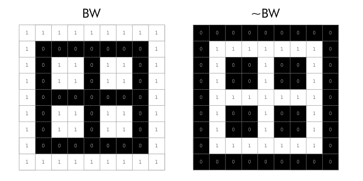Figure 6: Binary image composed of zeros and ones next to its inverse

Did you notice anything strange about gsSub?

The subtraction in the previous task inverted the intensities, so the text appears white and the background black. To restore the original order, invert the image again.

First, generate the binary image using imbinarize. Then invert the result using the NOT operator (~). Task Use imbinarize on gsSub without any options, and use the NOT operator (~) to invert the binary image. Store the result in BWsub and display it.

BWsub = ~imbinarize(gsSub);
imshow(BWsub)

Notice that with good preprocessing, adaptive thresholding wasn’t needed. The binarized image BWsub fully captures the text and little else.

Try computing the row sums for the binary images BW (which still has the background) and BWsub. Compare the row sums by plotting them on the same axes. Are there notable improvements?

The sequence of operations used here is very common: closing an image, then subtracting the original image from the closed image. It’s known as the “bottom hat transform,” and you can use the imbothat function in MATLAB to perform it. Try applying imbothat to gs using the structuring element SE.

BW = imbothat(gs,SE);

Binary Morphology

Enhancing Patterns 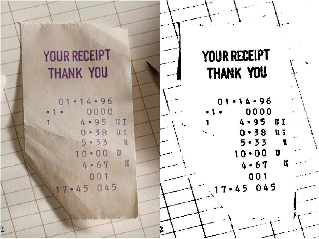Figure 7: Background subtraction doesn’t remove the grid.

The background subtraction process you used doesn’t remove the grid in the background of this receipt. The grid pattern is too thin to be included in the background generated by the closing operation.

Morphological operations are useful not only for removing features from an image but also for augmenting features. You can use morphology to enhance the text in the binary image and improve the row sum signal. Morphological opening expands the dark text regions, while closing diminishes them. Increasing the size of the structuring element increases these effects.

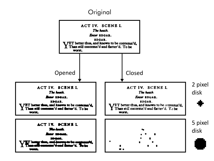Figure 8: Image of black text on white page with examples of morphological open and close operations on it.

To enhance a particular shape in an image, create a structural element in that shape. Here, you want to make each row of text a horizontal stripe, which looks like a short, wide rectangle.

You can create a rectangular structuring element using strel with a size array in the format [height width].

SE = strel("rectangle",[10 20]);

To determine the size of the rectangle, you can use features of a typical receipt. The rectangle should be short enough that the white space between rows of text is preserved, and it should be wide enough to connect adjacent letters. Task Use strel to create a rectangular structuring element with a height of 3 pixels and a width of 25 pixels. Store the result in SE.

SE = strel("rectangle",[3 25]);

In the previous section, to isolate the background, you eliminated the dark text by emphasizing the bright regions. To do this, you used imclose to close the image.

Here, emphasize the dark text instead, so perform the opposite operation and open the image using imopen.

Iopened = imopen(I,SE);

Using imopen with a wide rectangular structuring element turns lines of text into black horizontal stripes, which augments the valleys in the row sum signal. Task Apply a morphological opening operation to BW using the rectangular structuring element SE. Store the result in BWstripes and display it.

BWstripes = imopen(BW, SE);
imshow(BWstripes);

You can analyze whether the opening operation has improved the image processing algorithm by plotting the row sum. Task Sum the rows of BWstripes and store the result in S. Plot S to observe the row sum signal.

S = sum(BWstripes, 2);
plot(S)

The improvement is more noticeable if you plot the original row sum signal alongside the opened image row sum. Task Compute the row sum of the original signal BW and store the result in Sbw. Use hold on and hold off to add a plot of Sbw to your current plot.

hold on;
Sbw = sum(BW, 2);
plot(Sbw);
hold off;

The text rows generate more pronounced valleys after you enhanced them with the opening operation. There is also little to no loss of row definition from the opening operation because the rectangular structuring element was only three pixels high.

When using a very wide rectangular structuring element, there is a risk of amplifying valleys and peaks in the row sums of non-receipt images, which could lead to misclassifications. This risk is acceptable as long as the amplified row sum pattern in receipt images is more pronounced than the unwanted amplification in non-receipt images.

To see if this process generates unwanted valleys in a non-receipt image, you can apply the process to a new image by editing line 1 in the script:

I = imread("IMG_002.jpg");

Try testing the algorithm on IMG_005.jpg, IMG_008.jpg and IMG_013.jpg.