Matlab Image Processing Onramp: Introduction & Working with Images

Image Processing Onramp

Introduction

Course Overview

(1/2) Overview

Overview In Image Processing Onramp, you learn the fundamentals of image processing using MATLAB® and the Image Processing Toolbox®.

Many industries have image data, and image processing can help you get insights into that data. In this course, you get a hands-on learning experience where you implement an image processing workflow to identify images of receipts using MATLAB.

This course assumes basic knowledge of MATLAB. If you have never used MATLAB, or would like to refresh your skills, you can take MATLAB Onramp to get you up to speed quickly.

Hello, and welcome to Image Processing Onramp! Images are everywhere, in industries from healthcare to transportation, agriculture to retail, space exploration to archaeology, image data are used for monitoring, identification, and discovery. And where there are images, there is image processing.

At a high level, image processing is a set of techniques, which act on a digital image to modify it or extract information from it. Image processing techniques can be used to adjust contrast, remove noise, or find edges. And by combining multiple techniques, you can design algorithms which perform increasingly complex tasks.

In this course, you’ll use MATLAB and Image Processing Toolbox to implement a complete image processing workflow. By the end, you’ll have built an algorithm which can identify and collect images of receipts from a busy camera roll.

You don’t need to learn a lot of theory to start doing image processing, but it will help if you know a little bit of MATLAB—just the basics. If you’ve never used MATLAB before, it’s easy to get started, and we recommend you first take MATLAB Onramp to get you up to speed quickly. Throughout the course, you’ll be interacting with a web-based version of MATLAB inside our training environment. It has a slightly different look and feel from MATLAB Online or the desktop version of MATLAB, but don’t worry, you’re using the exact same MATLAB language. Enjoy the course!

(2/2) Learning Outcomes

What You Will Learn

In the next four modules, you learn and practice the following skills.

Images in MATLAB Import, display, and manipulate color and grayscale images.

Image Segmentation Create binary images by thresholding pixel intensity values.

Preprocessing and Postprocessing Techniques Improve image segmentation by using common preprocessing and postprocessing techniques.

Classification and Batch Processing Develop a metric to classify an image and apply that metric to a set of image files.

Receipt Identification Workflow

Throughout the course, you create an algorithm to identify images of receipts. As you learn the various image processing techniques, you apply them as part of the receipt identification workflow. Steps in the Receipt Identification Workflow

Figure 1: Receipt Identification Workflow

Images in MATLAB

Get Images into MATLAB

Import Images into MATLAB

In all MATLAB image processing workflows, the first step is to import images into the MATLAB workspace.

Once in the workspace, you can use MATLAB functions to display, process, and classify the images.

You can import an image into memory and assign it to a variable in the MATLAB workspace for later manipulation, display, and export.

A = imread("imgFile.jpg");

Ending the line with a semicolon stops MATLAB from displaying the values stored in A, which is helpful because images typically contain millions of values. Task Load image IMG_001.jpg into memory and assign it to variable I.

Remember to use a semicolon (;) so the values in I are not displayed.

I = imread("IMG_001.jpg");

In this course, you work with a mix of receipt and non-receipt images. The file names don’t indicate if an image is a receipt image, but you can find out by displaying the image.

Image data stored in a variable A can be displayed using the imshow function.

imshow(A)

Task Display the image data stored in I.

imshow(I)

To develop a robust classification algorithm, you’ll need additional images to analyze. Task Load IMG_002.jpg into the variable I2 and display it.

Remember to use a semicolon (;) when reading the image file.

I2 = imread("IMG_002.jpg");
imshow(I2)

You often want to view multiple images. For example, you might want to compare an image and a modified version of that image.

You can display two images together using the imshowpair function.

imshowpair(A1,A2,"montage")

The “montage” option places the images A1 and A2 side by side, with A1 on the left and A2 on the right. Task Display the images stored in I and I2 as a montage.

imshowpair(I, I2, "montage")

When you’re done processing an image in MATLAB, you can save it to a file. The function imwrite exports data stored in the MATLAB workspace to an image file.

imwrite(imgData,"img.jpg")

The output file format is automatically identified based on the file extension.

Try using imwrite to export I as a PNG file. Then use imread to load the image file into a new variable, and display it.

imwrite(I,"myImage.png")
Inew = imread("myImage.png");
imshow(Inew)

Remember that you can execute your script by clicking the Run button in the MATLAB Toolstrip.

When you’re ready, you can move on to the next section.

imwrite(I, "myImage.png")
Inew = imread("myImage.png")
imshow(Inew)

Grayscale and Color Images

(1/3) How Images are Stored in MATLAB

How Images are Stored in MATLAB When you bring an image into MATLAB, it is stored as a numeric array. Each pixel corresponds to an element in the array, with the array dimensions matching the image’s height and width in pixels. Grayscale images use integer values from 0 to 255 to represent pixel intensity, where low values indicate dark pixels and high values indicate bright pixels. Color images use three intensity values per pixel (red, green, and blue), forming a three-dimensional array with each color represented by a 2D matrix called a color plane. Viewing a color plane in grayscale shows the intensity of that particular color. For instance, bright regions of a red plane indicate pixels with a lot of red in them. When you bring an image into MATLAB, it’s stored as a numeric array. Each pixel corresponds to an element of the array. So the array has the same number of rows as the image’s height in pixels, and the same number of columns as the image’s width.

For a grayscale image, the numeric value for a pixel reflects the pixel’s intensity and can be any integer from 0 to 255. Dark pixels, like these, have low intensity values, while bright pixels have high intensity values.

Color images are also stored using intensities, but now each pixel has three intensity values: red, green, and blue, or RGB values. Each color’s intensity values are represented by a 2D matrix called a color plane. So even though the picture is two-dimensional, it’s stored as a three-dimensional array.

When you view a color plane, it’s displayed in grayscale. That’s because it’s a 2D matrix of intensities, just like a grayscale image. But since you know that this is the red color plane, you know that the bright pixels have a lot of red and the dark ones don’t. The blue color plane is pretty dark which tells us this image doesn’t have much blue in it. This bright patch here, well, it’s also bright in the green color plane. The result is a pale blue green in the color image. Different combinations of RGB values create the different colors you see in a color image.

(2/3) Extract Color Planes and Intensity Values

Color Planes

While receipts contain mostly grayscale colors, receipt images are still stored with three color planes like other color images. Like sunlight, which is composed of a full spectrum of colors, the color planes combine to create bright white paper.

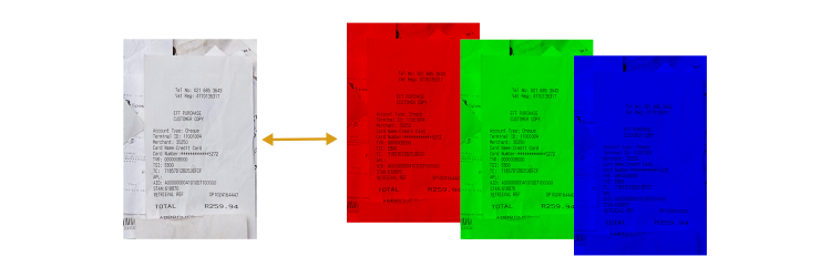Figure 2: Color planes explanation

Task Read IMG_003.jpg into the variable I, and then display it using imshow.

I = imread("IMG_003.jpg");
imshow(I)

Many image processing techniques are affected by image size. The images you’ll be classifying all have the same size: 600 pixels tall and 400 pixels wide.

You can find the size of an array by using the size function.

sz = size(A)

The size function returns a vector. The first element in the vector is the number of rows in the array, which corresponds to the height of the image. The second element is the number of columns in the array, which corresponds to the width of the image. Task Find the size of I and store the result in sz.

sz = size(I)

Did the size of the array match the size of the image in pixels? Almost. You probably noticed the additional element in the vector returned by the size function: 3.

The imported image is a color image, so that third element indicates the third dimension of the array, which stores the red, green, and blue color planes.

You can access individual color planes of an image by indexing into the third dimension. For example, you can extract the green (second) color plane using the value 2 as the third index.

Ig = I(:,:,2);

Task Extract the red color plane of the RGB image I and store it in R. Display R using imshow.

I1 = I(:, :, 1);
imshow(I1)
I2 = I(:, :, 2);
imshow(I2)
I3 = I(:, :, 3);
imshow(I3)

R = I1;
imshow(R);

Most images use the unsigned 8-bit integer (uint8) data type, which stores integers from 0 to 255. Bright or brightly colored images contain pixel intensity values near 255 in one or more color planes.

The red plane of this receipt image has some pretty bright areas. Do you think any elements of the red plane reach the maximum value of 255?

You can find the largest value in an array using the max function.

Amax = max(A,[],"all")

Using the “all” option finds the maximum across all values in the array. The brackets are required; they are placeholders for an unused input. Task Find the largest pixel intensity value of the red plane R and store the result in Rmax.

Rmax = max(R, [], "all")

Dark areas, like receipt text, contain values close to zero. Based on the image of the red plane from Task 3, do you think the red plane has any elements with a value of 0?

You can find the smallest value in an array using the min function.

Amin = min(A,[],"all")

Task Find the smallest pixel intensity value of the red plane and store the result in Rmin.

Rmin = min(R, [], "all")

Many common tasks can be completed more quickly using functions in Image Processing Toolbox. For example, to extract all three color planes of an image array, you can use imsplit instead of indexing into each plane individually.

[R,G,B] = imsplit(A);

You can display all three color planes at once by using the montage function.

montage({R,G,B})

Try using imsplit to extract the color planes of I. Then display all three color planes using montage.

When you’re ready, you can move on to the next section.

(3/3) Convert from Color to Grayscale

Why Convert to Grayscale?

When loaded into memory, a grayscale image occupies a third of the space required for an RGB image. Because a grayscale image has a third of the data, it requires less computational power to process and can reduce computation time. A grayscale image is conceptually simpler than an RGB image, so developing an image processing algorithm can be more straightforward when working with grayscale.

In receipt images, like the one shown below, little information is lost when converting to grayscale. The essential characteristics, like the dark text and bright paper, are preserved.

On the other hand, if you wanted to classify the produce visible in the background, the color planes are essential. After converting to grayscale, it’s hard to see the broccoli, let alone classify it.

Color image of a receipt with produce in the background, next to the same image in grayscale. 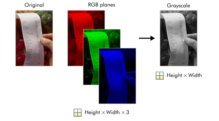Figure 3: Color vs Grayscale Receipt

The algorithm you implement in this course is built around identifying text, so color is not necessary. Converting the images to grayscale eliminates color and helps the algorithm focus on the black-and-white patterns found in receipts.

You can convert an image to grayscale using the im2gray function.

Ags = im2gray(A);

Task Convert the RGB image I to a grayscale image and store the result in gs. Display gs.

gs = im2gray(I);
imshow(gs)

Did you notice that the purple color of the receipt text is lost during the conversion to grayscale? Because not all receipts have purple text, the purple values aren’t useful in a classification algorithm.

This negligible loss of information has a benefit: gs is one third the size of I, having only two dimensions instead of three. You can verify the size with the size function. Task Find the size of gs and store the result in sz.

sz = size(gs)

The grayscale image created by im2gray is a single plane of intensity values. The intensity values are computed as a weighted sum of the RGB planes. For more information about grayscale conversion, see the documentation for im2gray.

If you need your converted grayscale images later, you can save them to a file. Try using imwrite to save gs to the file gs.jpg.

Contrast Adjustment

Contrast and Intensity Histograms

Even though these two receipt images are grayscale, the contrast is different.

If you are analyzing a set of images, normalizing the brightness can be an important preprocessing step, especially for identifying the black-and-white patterns of text in receipt images. A grayscale image of a receipt next to a darker image of a receipt with low contrast

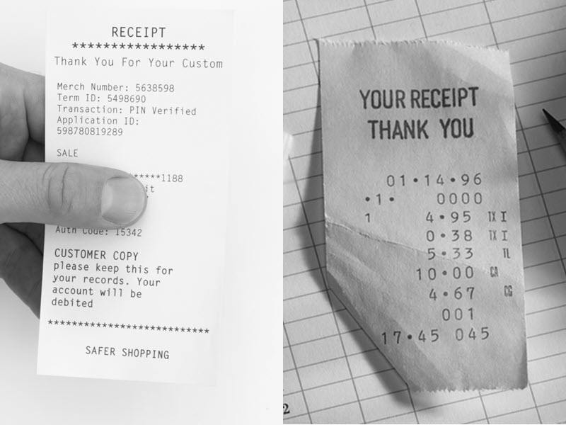Figure 4: Receipt Contrast Comparison

An intensity histogram separates pixels into bins based on their intensity values. Dark images, for example, have many pixels binned in the low end of the histogram. Bright images have many pixels binned at the high end of the histogram.

The histogram often suggests where simple adjustments can be made to improve the definition of image features. Do you notice any adjustments that could be made to the receipt image so that the text is easier to identify?

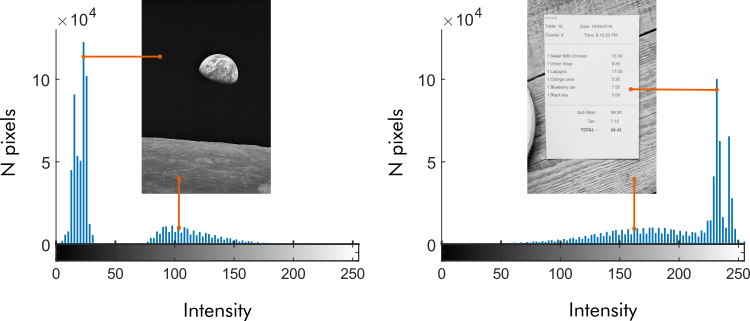Figure 5: Receipt Histogram

One of the essential identifying features of a receipt image is text. Receipt images should have good contrast so that the text stands out from the paper background.

You can investigate the contrast in an image by viewing its intensity histogram using the imhist function.

imhist(I)

If the histogram shows pixels binned mainly at the high and low ends of the spectrum, then the receipt has good contrast. If not, it could probably benefit from a contrast adjustment. Task Display the intensity histogram for the grayscale image gs.

imhist(gs)

Did the histogram of gs suggest high contrast between the receipt text and paper, or do you believe it could use an adjustment?

A second image, gs2, is displayed in the script. Does it appear washed out? While a visual inspection can be useful, it’s often easier to assess the contrast by viewing the histogram. Task Display the intensity histogram for gs2.

imhist(gs2)

The intensity histogram of gs2 shows lower contrast between the text and the background. Most of the dark pixels have intensity values around 100, and not many bright pixels have intensity values above 200. So, the contrast is about half of what it could be if the image used the full intensity range (0 to 255).

Increasing image contrast brightens brighter pixels and darkens darker pixels. You can use the imadjust function to adjust the contrast of a grayscale image automatically.

Aadj = imadjust(A);

Task Adjust the contrast of gs2 and save the result in gs2Adj.

Display gs2 and gs2Adj side by side using the imshowpair function with the “montage” option.

gs2Adj = imadjust(gs2);
imshowpair(gs2Adj,gs2,"montage")

The histogram of the adjusted image reflects the changes made by imadjust. Darker pixels have shifted to lower bins, while brighter pixels have shifted to higher bins. Task Display the intensity histogram for gs2Adj.

imhist(gs2Adj)

Did imadjust work well to improve the contrast of gs2 so the text stands out? If not, what further adjustments would you make?

Try adjusting the contrast of gs and displaying the adjusted histogram. Does imadjust work well here, too?

imadjust works only for grayscale images unless you provide additional inputs to the function. You can, however, use the function imlocalbrighten to adjust the contrast of a color image. Try using imlocalbrighten on the color image I2 and display the result.

I2adj = imlocalbrighten(I2);

When you’re ready, you can move on to the next section.

Work with Images Interactively

(1/2) The Image Viewer App

The Image Viewer App The Image Viewer app is a useful tool to inspect images. The Image Viewer app offers a point-and-click interface for image inspection and adjustment. Open the Image Viewer app using the imageViewer command or from the Apps tab. The app allows you to view image information, inspect pixels, and adjust grayscale contrast interactively. So far, you’ve used MATLAB to read and display images, inspect their properties, plot their intensity histograms, and adjust their contrast, all using MATLAB commands. Prefer a point-and-click approach? Well, try the Image Viewer app. You can use the app to display the image, view information, and display the intensity histogram to interactively adjust the contrast.

Open the Image Viewer app using the command imageViewer, or by going to the Apps tab, selecting the drop-down, and searching for Image Viewer.

Let’s start by clicking Import Image to load and view an image of a highway at night. You can click Image Metadata to display information about the image like the size or data type.

To inspect the RGB values of the image, click Zoom To Pixels. Image Overview displays the full image with a box indicating that these pixels came from a section of road in the middle of the picture. These dark road pixels have low intensity values and contain a bit more blue than red or green. You can move the Region Selector with your mouse or with the arrow keys to inspect another area. The tail lights have higher red values.

Let’s inspect a grayscale image by importing a picture of a receipt from the workspace. Now when we inspect the pixels with Zoom To Pixels, we only see one intensity value. You can interactively adjust contrast in a grayscale image using an interactive histogram. Adjust the left slider to augment dark pixels, and adjust the right slider to brighten lighter pixels.

When you’re done, you can export the image to the workspace or save it to a file.

(2/2) Explore Images Interactively

Two images have been loaded into the workspace: gs2 and sunset. Use the command imageViewer to open the Image Viewer app and explore the two images.

Remember that you can execute your script by clicking the Run or Run Section button in the MATLAB Toolstrip.

As you explore, try some of these tasks: Import the image sunset from the workspace and inspect pixel values by selecting Zoom To Pixels. Explore various areas of the image by moving the region. You can do this by panning or by opening Image Overview and dragging the box to a new location. What do you notice about the RGB values in brightly colored regions? What about dark regions or regions that are nearly white? Import the image gs2 from the workspace and inspect its pixel values. You automatically adjusted the contrast of gs2 in the previous section using imadjust. You probably noticed that the image could benefit from additional contrast enhancement. Adjust the contrast of gs2 using the Interactive Histogram tool in the Contrast tab to provide the best possible text definition. When you’re satisfied with the image contrast, export the enhanced image to the workspace or a file.

When you’re ready, close the Image Viewer app and move on to the next section.